Neural Networks and Deep Learning
See how inputs, weights, layers, and feedback turn numbers into a prediction.
A network is a set of calculations
A neural network connects mathematical units in layers. A unit, often called a neuron, combines values and passes a result onwards. The name comes from a loose inspiration from biology. It is not a faithful copy of a brain cell.
The input layer receives the model’s input values. Hidden layers transform them. The output layer produces a result, such as scores for possible categories. “Hidden” means between input and output; it does not mean encrypted or secret.
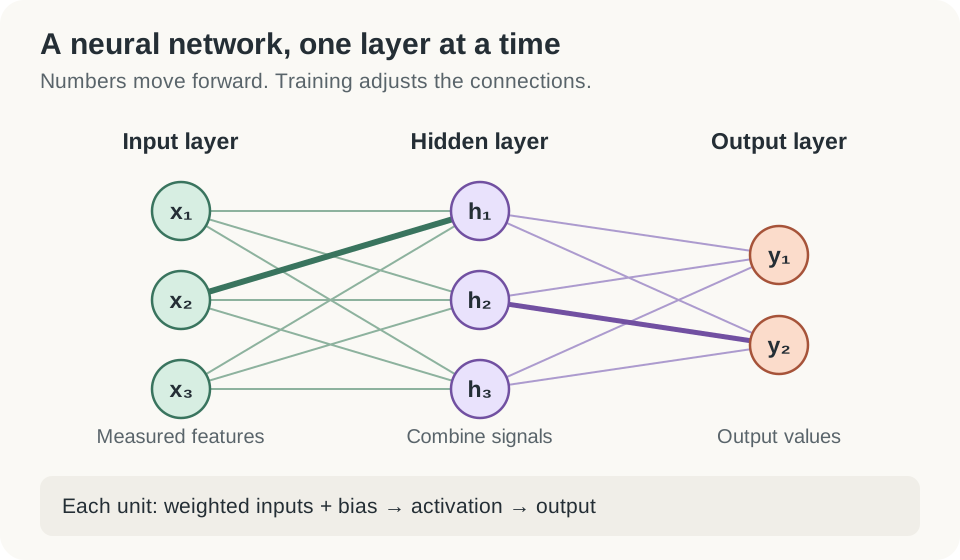
Open the diagram for a larger view.
Follow the arrows from left to right. This is a simplified network illustration; real designs vary.
Weights, bias, and activation
A weight is a learned number that controls how an input contributes to a calculation. A bias is another learned number that shifts the result. Here “bias” is a mathematical term, separate from unfair treatment of people.
Consider an imaginary unit with two inputs:
combined value = (input A × weight A) + (input B × weight B) + bias
If A is 2, B is 1, the weights are 0.5 and −1, and the bias is 0.2, the combined value is 0.2. This small example shows the arithmetic; those numbers are not a trained security detector.
Google’s nodes and hidden layers lesson lets you explore this calculation visually.
An activation function changes the combined value before it moves onwards. Many activations add a non-straight-line relationship, called nonlinearity. That lets networks represent more complicated patterns. One simple activation, ReLU, returns zero for a negative value and keeps a positive value unchanged. See Google’s activation lesson.
How learning changes the network
The network first makes a prediction. A loss function measures how far that prediction is from the training target. Backpropagation calculates how changes in the model’s parameters would affect the loss. An optimizer then adjusts the parameters, usually in small steps.
The sequence is: predict → measure error → calculate gradients → update → repeat. A gradient describes how the loss changes when a parameter changes. A learning rate controls the size of an update.
Imagine adjusting sound controls to match a recording. You need feedback about the mismatch and a way to choose adjustments. A network uses mathematics for those steps.
The PyTorch optimization tutorial shows a real training loop. Google’s backpropagation explanation offers another learning route.
What makes learning “deep”?
Deep learning uses neural networks with multiple processing layers. Layers can learn useful combinations of simpler patterns. In an image system, these may progress from simple visual features towards more complex ones. There is no single universal layer-count rule worth memorising here.
Deep learning can use labelled data. It can also use self-supervised or other learning approaches. Depth describes the network; supervised or self-supervised describes the learning setup. These answer different questions.
A large network can still make mistakes or learn shortcuts. More layers do not establish that a prediction is safe. PyTorch’s labelled image-classification example is a practical demonstration that neural-network learning and labels can work together.
Check your understanding
Does backpropagation itself decide and apply every parameter update?
No. Backpropagation calculates gradients. The optimizer uses those gradients and its update rule to change parameters. Keeping these steps separate makes the training process easier to understand.